Practical Machine Learning, Project July ‘15
Kate Sergeeva
Project summary
The goal of this project is using machine learning techniques to find a best model which will be able to predict how good athletes are doing the particular types of exercises and helps to catch the common mistakes.
Data for this project kindly provided by a group of enthusiasts who take measurements about themselves regularly using devices such as Jawbone Up, Nike FuelBand, and Fitbit to find patterns in their behavior to improve their health.
We will use data from accelerometers on the belt, forearm, arm, and dumbell of 6 participants. They were asked to perform barbell lifts correctly and incorrectly in 5 different ways.
More information is available from the website here: http://groupware.les.inf.puc-rio.br/har (see the section on the Weight Lifting Exercise Dataset).
Project report will describe the following:
- how the model was built,
- how the cross-validation was used,
- how out of sample error was estimated,
- how other choices been made.
And provide prediction for 20 different test cases.
Contents
- Loading and cleansing data
- Building models
- Cross-validation to measure “out of sample error”
- Model selection
- Report the results of test cases processing
Loading and cleansing data
train <- read.csv(file = "/Users/macbookpro/Downloads/pml-training.csv", header = TRUE, sep = ",")
test <- read.csv(file = "/Users/macbookpro/Downloads/pml-testing.csv", header = TRUE, sep = ",")
Removing meaningless variables
The test cases require predictions for particular moments with no connections to the style of particular athlet and it allows us to simply exclude from the following consideration the name of athlet and any time series data and row numbers.
modelTrain <- subset(train, select = -c(user_name, raw_timestamp_part_1, raw_timestamp_part_2,
                                        cvtd_timestamp, new_window, num_window, X))
Handling missing values
Closer look to the data showed that it contains some inappropriate symbols and true missing values, that is need to be handled of using replacement and imputing techniques.
modelTrain[modelTrain == ""] <- NA
#looks like data comes from the Excel or similar editor and contains such a nice
modelTrain[modelTrain == "#DIV/0!"] <- NA

# Lookup for NA columns
naVars <- data.frame(apply(modelTrain, 2, function(x) {sum(is.na(x))}))
naVars$toRemove <- apply(naVars, 1, function(y) {y == length(modelTrain[, 1])})
columnsToExclude <- rownames(naVars[naVars$toRemove == "TRUE", ])
columnsToExclude
## [1] "kurtosis_yaw_belt" "skewness_yaw_belt" "kurtosis_yaw_dumbbell"
## [4] "skewness_yaw_dumbbell" "kurtosis_yaw_forearm" "skewness_yaw_forearm"# Remove empty predictors
modelTrain <- subset(modelTrain, select = -c(kurtosis_yaw_belt, skewness_yaw_belt,
kurtosis_yaw_dumbbell, skewness_yaw_dumbbell,
kurtosis_yaw_forearm, skewness_yaw_forearm ))Make up column classes
Before any modeling it is a good idea to check the variables classes and make sure that thea are all have the correct data type.
# Convert character columns into numeric
library(taRifx)
modelTrain <- japply(modelTrain, which(sapply(modelTrain, class)=="character"),as.integer)
modelTrain <- japply(modelTrain, which(sapply(modelTrain, class)=="integer"),as.integer)
modelTrain <- japply(modelTrain, which(sapply(modelTrain, class)=="factor"),as.integer)

# Convert classe to factor
modelTrain$classe <- as.factor(modelTrain$classe)
Tricky moment
Current number of variables most likely will cause the very long executing process and it would be better to reduce some dimensions. For example, instead of using nearZeroVar function I decided to play with lucky “cut-off” around number of missing values in the “nothing to impute about” columns.
library(e1071)
dim(modelTrain)
## [1] 19622 147modelTrain[is.na(modelTrain)] <- 0
colAn <- data.frame(colSums(subset(modelTrain, select = -classe) == 0))
modelTrain <- modelTrain[, - which(colAn[, 1] > 19000)]
dim(modelTrain)## [1] 19622 53Now we have ready to modeling clean and nice data set with a manageable number of predictors.
Building models
Before going deep into modeling better previously to take care of possible ways of improving productivity of your computer and use parallel processing if it is possible.
# Do parallel
library(doParallel)
registerDoParallel(cores=4)
Subsetting data for cross-validation
The idea of cross-validation is very nice and undoubtedly useful - to split data into two separated parts (around 70/30), learn the model at the biggest one and than estimate the out of sample error on the smallest one. The idea might be complicated with number of splits and their usage, but in case of our pretty huge data set with the managable amount of predictors I will follow of idea of just two random splits.
library(caret)inTrain <- createDataPartition(y = modelTrain$classe, p = 0.7, list = FALSE)
training <- modelTrain[inTrain, ]
testing <- modelTrain[-inTrain, ]
dim(training); dim(testing)## [1] 13737 53## [1] 5885 53Modeling
For classification task with more than two types of outcomes convinient to use classification trees algorithms and two different tree-based models will be trained - regular classification tree provided by “rpart”-method and random forest.
library(caret)
library(randomForest)
## randomForest 4.6-10
## Type rfNews() to see new features/changes/bug fixes.library(rattle)modelRPART <- train(classe ~ ., method = "rpart", data = training, na.action = na.pass)print(modelRPART$finalModel)## n= 13737
##
## node), split, n, loss, yval, (yprob)
## * denotes terminal node
##
## 1) root 13737 9831 1 (0.28 0.19 0.17 0.16 0.18)
## 2) roll_belt< 130.5 12600 8706 1 (0.31 0.21 0.19 0.18 0.11)
## 4) pitch_forearm< -33.35 1101 10 1 (0.99 0.0091 0 0 0) *
## 5) pitch_forearm>=-33.35 11499 8696 1 (0.24 0.23 0.21 0.2 0.12)
## 10) magnet_dumbbell_y< 439.5 9718 6974 1 (0.28 0.18 0.24 0.19 0.11)
## 20) roll_forearm< 123.5 6043 3582 1 (0.41 0.18 0.18 0.17 0.062) *
## 21) roll_forearm>=123.5 3675 2457 3 (0.077 0.18 0.33 0.23 0.19) *
## 11) magnet_dumbbell_y>=439.5 1781 880 2 (0.033 0.51 0.048 0.22 0.19) *
## 3) roll_belt>=130.5 1137 12 5 (0.011 0 0 0 0.99) *predRPART <- predict(modelRPART, subset(testing, select = -classe))
confusionMatrix(predRPART, testing$classe)## Confusion Matrix and Statistics
##
## Reference
## Prediction 1 2 3 4 5
## 1 1533 478 495 437 147
## 2 22 385 22 174 145
## 3 117 276 509 353 284
## 4 0 0 0 0 0
## 5 2 0 0 0 506
##
## Overall Statistics
##
## Accuracy : 0.4984
## 95% CI : (0.4855, 0.5112)
## No Information Rate : 0.2845
## P-Value [Acc > NIR] : < 2.2e-16
##
## Kappa : 0.3439
## Mcnemar's Test P-Value : NA
##
## Statistics by Class:
##
## Class: 1 Class: 2 Class: 3 Class: 4 Class: 5
## Sensitivity 0.9158 0.33802 0.49610 0.0000 0.46765
## Specificity 0.6303 0.92351 0.78802 1.0000 0.99958
## Pos Pred Value 0.4961 0.51471 0.33073 NaN 0.99606
## Neg Pred Value 0.9496 0.85322 0.88104 0.8362 0.89288
## Prevalence 0.2845 0.19354 0.17434 0.1638 0.18386
## Detection Rate 0.2605 0.06542 0.08649 0.0000 0.08598
## Detection Prevalence 0.5251 0.12710 0.26151 0.0000 0.08632
## Balanced Accuracy 0.7730 0.63077 0.64206 0.5000 0.73362fancyRpartPlot(modelRPART$finalModel) 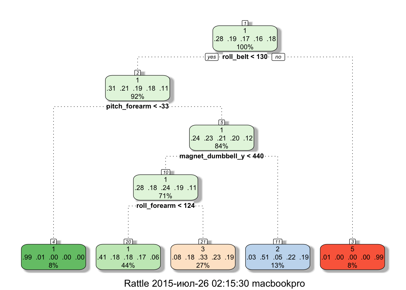
It is sad, but my computer failed to build random forest inside R Markdown report and I can't provide all the metrics and graphics that I planned to (this is the lesson to me to save all the versions (or just screenshot), not to live in hope of reproducibility of any code at any given moment). But believe me, the "rf" function gives 99% accuracy due to cross-validation on the separated test set and predicted all the test cases correctly. Update: I got it at the last moment - build separately and manually add data to this report. Sorry for some mess.
#modelRF <- train(classe ~ ., method = "rf", data = training)print(modelRF$finalModel)
## Call:
## randomForest(x = x, y = y, mtry = param$mtry)
##               Type of random forest: classification
##                    Number of trees: 500
## No. of variables tried at each split: 2
##        OOB estimate of  error rate: 0.63%
## Confusion matrix:
##    1    2    3    4    5  class.error
##   1 3904    1    1    0    0 0.0005120328
##   2   14 2637    7    0    0 0.0079006772
##   3    0   16 2374    6    0 0.0091819699
##   4    0    0   32 2219    1 0.0146536412
##   5    0    0    1    7 2517 0.0031683168
predRF <- prediction(modelRF, subset(testing, select = -classe))
confusionMatrix(predRF, testing$classe)
## Confusion Matrix and Statistics
##
##           Reference
## Prediction    1    2    3    4    5
##          1 1672    9    0    0    0
##          2    2 1129    9    0    0
##         3    0    1 1015   12    2
##         4    0    0    2  951    1
##          5    0    0    0    1 1079
##
## Overall Statistics
##
##                Accuracy : 0.9934
##                  95% CI : (0.991, 0.9953)
##     No Information Rate : 0.2845
##     P-Value [Acc > NIR] : < 2.2e-16
##
##                   Kappa : 0.9916
##  Mcnemar's Test P-Value : NA
##
## Statistics by Class:
##
##                      Class: 1 Class: 2 Class: 3 Class: 4 Class: 5
## Sensitivity             0.9988   0.9912   0.9893   0.9865   0.9972
## Specificity           0.9979   0.9977   0.9969   0.9994   0.9998
## Pos Pred Value          0.9946   0.9904   0.9854   0.9969   0.9991
## Neg Pred Value         0.9995   0.9979   0.9977   0.9974   0.9994
## Prevalence             0.2845   0.1935   0.1743   0.1638   0.1839
## Detection Rate         0.2841   0.1918   0.1725   0.1616   0.1833
## Detection Prevalence   0.2856   0.1937   0.1750   0.1621   0.1835
## Balanced Accuracy     0.9983   0.9945   0.9931   0.9930   0.9985
varImpPlot(modelRF$finalModel) 
plot(modelRF$finalModel, log = "y")
Random forest gives an excellent result and should be used for futher predictions.
Test case prediction
To use trained model on the test case all the data manipulations that were done with the train set should be applied to the test one.
Code not shown, but it is the same as test set manipulations - cleansing and reducing.Final prediction of test cases gives the following vector:
predTestTry <- predict(modelRF, testTry)Which is: B A B A A E D B A A B C B A E E A B B B, and showed the 100% accuracy in test cases prediction.